!pip install ucimlrepoLinear regression example
import numpy as np
import pandas as pd
import matplotlib.pyplot as plt

from ucimlrepo import fetch_ucirepo
from sklearn.model_selection import train_test_split
from sklearn.linear_model import LinearRegression
# fetch dataset
dataset = fetch_ucirepo(id=1) # abalone dataset
# metadata
print(dataset.metadata)
# variable information
print(dataset.variables){'uci_id': 1, 'name': 'Abalone', 'repository_url': 'https://archive.ics.uci.edu/dataset/1/abalone', 'data_url': 'https://archive.ics.uci.edu/static/public/1/data.csv', 'abstract': 'Predict the age of abalone from physical measurements', 'area': 'Biology', 'tasks': ['Classification', 'Regression'], 'characteristics': ['Tabular'], 'num_instances': 4177, 'num_features': 8, 'feature_types': ['Categorical', 'Integer', 'Real'], 'demographics': [], 'target_col': ['Rings'], 'index_col': None, 'has_missing_values': 'no', 'missing_values_symbol': None, 'year_of_dataset_creation': 1994, 'last_updated': 'Mon Aug 28 2023', 'dataset_doi': '10.24432/C55C7W', 'creators': ['Warwick Nash', 'Tracy Sellers', 'Simon Talbot', 'Andrew Cawthorn', 'Wes Ford'], 'intro_paper': None, 'additional_info': {'summary': 'Predicting the age of abalone from physical measurements. The age of abalone is determined by cutting the shell through the cone, staining it, and counting the number of rings through a microscope -- a boring and time-consuming task. Other measurements, which are easier to obtain, are used to predict the age. Further information, such as weather patterns and location (hence food availability) may be required to solve the problem.\r\n\r\nFrom the original data examples with missing values were removed (the majority having the predicted value missing), and the ranges of the continuous values have been scaled for use with an ANN (by dividing by 200).', 'purpose': None, 'funded_by': None, 'instances_represent': None, 'recommended_data_splits': None, 'sensitive_data': None, 'preprocessing_description': None, 'variable_info': 'Given is the attribute name, attribute type, the measurement unit and a brief description. The number of rings is the value to predict: either as a continuous value or as a classification problem.\r\n\r\nName / Data Type / Measurement Unit / Description\r\n-----------------------------\r\nSex / nominal / -- / M, F, and I (infant)\r\nLength / continuous / mm / Longest shell measurement\r\nDiameter\t/ continuous / mm / perpendicular to length\r\nHeight / continuous / mm / with meat in shell\r\nWhole weight / continuous / grams / whole abalone\r\nShucked weight / continuous\t / grams / weight of meat\r\nViscera weight / continuous / grams / gut weight (after bleeding)\r\nShell weight / continuous / grams / after being dried\r\nRings / integer / -- / +1.5 gives the age in years\r\n\r\nThe readme file contains attribute statistics.', 'citation': None}}
name role type demographic \
0 Sex Feature Categorical None
1 Length Feature Continuous None
2 Diameter Feature Continuous None
3 Height Feature Continuous None
4 Whole_weight Feature Continuous None
5 Shucked_weight Feature Continuous None
6 Viscera_weight Feature Continuous None
7 Shell_weight Feature Continuous None
8 Rings Target Integer None
description units missing_values
0 M, F, and I (infant) None no
1 Longest shell measurement mm no
2 perpendicular to length mm no
3 with meat in shell mm no
4 whole abalone grams no
5 weight of meat grams no
6 gut weight (after bleeding) grams no
7 after being dried grams no
8 +1.5 gives the age in years None no # data (as pandas dataframes)
X = dataset.data.features
y = dataset.data.targets
print(X.shape, y.shape)(4177, 8) (4177, 1)X.head()| Sex | Length | Diameter | Height | Whole_weight | Shucked_weight | Viscera_weight | Shell_weight | |
|---|---|---|---|---|---|---|---|---|
| 0 | M | 0.455 | 0.365 | 0.095 | 0.5140 | 0.2245 | 0.1010 | 0.150 |
| 1 | M | 0.350 | 0.265 | 0.090 | 0.2255 | 0.0995 | 0.0485 | 0.070 |
| 2 | F | 0.530 | 0.420 | 0.135 | 0.6770 | 0.2565 | 0.1415 | 0.210 |
| 3 | M | 0.440 | 0.365 | 0.125 | 0.5160 | 0.2155 | 0.1140 | 0.155 |
| 4 | I | 0.330 | 0.255 | 0.080 | 0.2050 | 0.0895 | 0.0395 | 0.055 |
y.head()| Rings | |
|---|---|
| 0 | 15 |
| 1 | 7 |
| 2 | 9 |
| 3 | 10 |
| 4 | 7 |
# Convert categorical 'Sex' using get_dummies()
X = pd.get_dummies(X)
X.head()| Length | Diameter | Height | Whole_weight | Shucked_weight | Viscera_weight | Shell_weight | Sex_F | Sex_I | Sex_M | |
|---|---|---|---|---|---|---|---|---|---|---|
| 0 | 0.455 | 0.365 | 0.095 | 0.5140 | 0.2245 | 0.1010 | 0.150 | False | False | True |
| 1 | 0.350 | 0.265 | 0.090 | 0.2255 | 0.0995 | 0.0485 | 0.070 | False | False | True |
| 2 | 0.530 | 0.420 | 0.135 | 0.6770 | 0.2565 | 0.1415 | 0.210 | True | False | False |
| 3 | 0.440 | 0.365 | 0.125 | 0.5160 | 0.2155 | 0.1140 | 0.155 | False | False | True |
| 4 | 0.330 | 0.255 | 0.080 | 0.2050 | 0.0895 | 0.0395 | 0.055 | False | True | False |
# Convert to numpy arrays
X_np = X.to_numpy().astype('float')
y_np = y.to_numpy().flatten()

# Split into train and test sets
X_train, X_test, y_train, y_test = train_test_split(X_np, y_np, test_size=0.2, random_state=42)
X_train, X_val, y_train, y_val = train_test_split(X_train, y_train, test_size=0.2, random_state=42)

print(f'Samples for training: {X_train.shape[0]}')
print(f'Samples for validation: {X_val.shape[0]}')
print(f'Samples for testing: {X_test.shape[0]}')
Samples for training: 2672
Samples for validation: 669
Samples for testing: 836# Fit regression model
model = LinearRegression()
model.fit(X_train, y_train)
# Evaluate
score = model.score(X_test, y_test)
print(f"Test R^2: {score:.3f}")
print("Coefficients:", model.coef_)Test R^2: 0.545
Coefficients: [ -1.02217201 8.83603361 24.35454601 8.94974547 -20.65659391
-9.05850108 7.59042072 0.19513526 -0.50004446 0.3049092 ]N_train = X_train.shape[0]
N_val = X_val.shape[0]
N_test = X_test.shape[0]
theta = np.random.rand(X_train.shape[1])
eta = 1e-5
nepochs = 10000
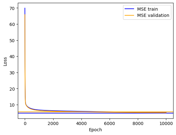
mse_train = []
mse_val = []
for epoch in range(nepochs + 1):
theta = theta + eta * X_train.T @ (y_train - X_train @ theta)
mse_train.append((1/N_train) * np.linalg.norm(y_train - X_train @ theta)**2)
mse_val.append((1/N_val) * np.linalg.norm(y_val - X_val @ theta)**2)
# Analytical solution
theta_analytical = np.linalg.inv(X_train.T @ X_train) @ X_train.T @ y_train
mse_analytical_train = (1/N_train) * np.linalg.norm(y_train - X_train @ theta_analytical)**2
mse_analytical_val = (1/N_val) * np.linalg.norm(y_val - X_val @ theta_analytical)**2
plt.plot(mse_train, label='MSE train', color='blue')
plt.axhline(y=mse_analytical_train, xmin=0, xmax=1, color='blue')
plt.plot(mse_val, label='MSE validation', color='orange')
plt.axhline(y=mse_analytical_val, xmin=0, xmax=1, color='orange')
plt.xlabel('Epoch')
plt.ylabel('Loss')
plt.legend()
plt.show()