%matplotlib inline
import matplotlib.pyplot as plt
import numpy as np

from skimage.io import imread
from skimage.transform import resizeConvolución en Keras
Este notebook muestra la aplicación de convoluciones en imágenes.
Descargas
Lectura y apertura de imágenes
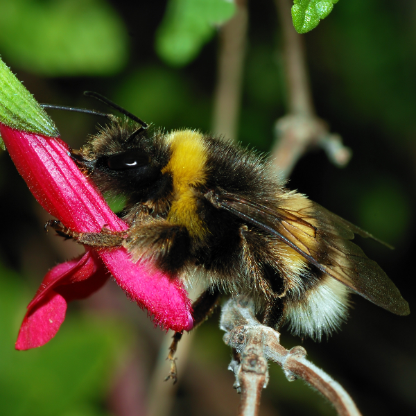
El siguiente código permite leer una imagen, cargarla en un arreglo de numpy y mostrarla.
sample_image = imread("bee.png").astype("float32")
print("sample image shape: ", sample_image.shape)

size = sample_image.shape

plt.imshow(sample_image.astype('uint8'));
sample image shape: (600, 600, 3)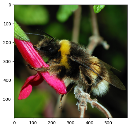
Filtro de convolución
El objetivo de esta sección es utilizar TensorFlow / Keras para realizar convoluciones individuales sobre imágenes. En esta sección todavía no se entrena ningún modelo.
import tensorflow as tf

print(tf.__version__)2.16.2from tensorflow.keras.models import Sequential
from tensorflow.keras.layers import Conv2Dconv = Conv2D(filters=3, kernel_size=(5, 5), padding="same")sample_image.shape(600, 600, 3)img_in = np.expand_dims(sample_image, 0)
img_in.shape(1, 600, 600, 3)Si aplicamos esta convolución a esta imagen, ¿cuál será la forma del mapa de características generado?
Pistas:
- En Keras
padding="same"significa que las convoluciones usan el relleno necesario para preservar la dimensión espacial de las imágenes o mapas de entrada.
- En Keras, las convoluciones no tienen strides por defecto.
- ¿Cuánto padding debe usar Keras en este caso particular para preservar las dimensiones espaciales?
img_out = conv(img_in)
print(type(img_out), img_out.shape)
<class 'tensorflow.python.framework.ops.EagerTensor'> (1, 600, 600, 3)La salida puede convertirse a un arreglo de numpy
np_img_out = img_out[0].numpy()
print(type(np_img_out))
<class 'numpy.ndarray'>fig, (ax0, ax1) = plt.subplots(ncols=2, figsize=(10, 5))
ax0.imshow(sample_image.astype('uint8'))
ax1.imshow(np_img_out.astype('uint8'));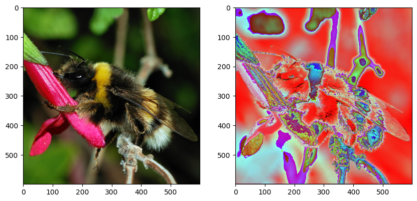
La salida tiene 3 canales, por lo tanto, también puede interpretarse como una imagen RGB con matplotlib. Sin embargo, es el resultado de un filtro convolucional aleatorio aplicado a la imagen original.
Veamos los parámetros:
conv.count_params()228Pregunta: ¿Puedes calcular el número de parámetros entrenables a partir de los hiperparámetros de la capa?
Pistas:
- la imagen de entrada tiene 3 colores y un único kernel de convolución mezcla información de los tres canales de entrada para calcular su salida;
- una capa convolucional genera muchos canales de salida a la vez: cada canal es el resultado de una operación de convolución distinta (también llamada unidad) de la capa;
- No olvidar los sesgos/biases
len(conv.get_weights())2weights = conv.get_weights()[0]
weights.shape(5, 5, 3, 3)Cada uno de los 3 canales de salida es generado por un kernel de convolución distinto.
Cada kernel tiene dimensión 5x5 y opera sobre los 3 canales de entrada.
biases = conv.get_weights()[1]
biases.shape(3,)Un bias por canal de salida.
Podemos construir un kernel nosotros mismos (“manualmente”).
def my_init(shape=(5, 5, 3, 3), dtype=None):
    array = np.zeros(shape=shape, dtype="float32")
    array[:, :, 0, 0] = 1 / 25
    array[:, :, 1, 1] = 1 / 25
    array[:, :, 2, 2] = 1 / 25
    return array
np.transpose(my_init(), (2, 3, 0, 1))array([[[[0.04, 0.04, 0.04, 0.04, 0.04],
[0.04, 0.04, 0.04, 0.04, 0.04],
[0.04, 0.04, 0.04, 0.04, 0.04],
[0.04, 0.04, 0.04, 0.04, 0.04],
[0.04, 0.04, 0.04, 0.04, 0.04]],
[[0. , 0. , 0. , 0. , 0. ],
[0. , 0. , 0. , 0. , 0. ],
[0. , 0. , 0. , 0. , 0. ],
[0. , 0. , 0. , 0. , 0. ],
[0. , 0. , 0. , 0. , 0. ]],
[[0. , 0. , 0. , 0. , 0. ],
[0. , 0. , 0. , 0. , 0. ],
[0. , 0. , 0. , 0. , 0. ],
[0. , 0. , 0. , 0. , 0. ],
[0. , 0. , 0. , 0. , 0. ]]],
[[[0. , 0. , 0. , 0. , 0. ],
[0. , 0. , 0. , 0. , 0. ],
[0. , 0. , 0. , 0. , 0. ],
[0. , 0. , 0. , 0. , 0. ],
[0. , 0. , 0. , 0. , 0. ]],
[[0.04, 0.04, 0.04, 0.04, 0.04],
[0.04, 0.04, 0.04, 0.04, 0.04],
[0.04, 0.04, 0.04, 0.04, 0.04],
[0.04, 0.04, 0.04, 0.04, 0.04],
[0.04, 0.04, 0.04, 0.04, 0.04]],
[[0. , 0. , 0. , 0. , 0. ],
[0. , 0. , 0. , 0. , 0. ],
[0. , 0. , 0. , 0. , 0. ],
[0. , 0. , 0. , 0. , 0. ],
[0. , 0. , 0. , 0. , 0. ]]],
[[[0. , 0. , 0. , 0. , 0. ],
[0. , 0. , 0. , 0. , 0. ],
[0. , 0. , 0. , 0. , 0. ],
[0. , 0. , 0. , 0. , 0. ],
[0. , 0. , 0. , 0. , 0. ]],
[[0. , 0. , 0. , 0. , 0. ],
[0. , 0. , 0. , 0. , 0. ],
[0. , 0. , 0. , 0. , 0. ],
[0. , 0. , 0. , 0. , 0. ],
[0. , 0. , 0. , 0. , 0. ]],
[[0.04, 0.04, 0.04, 0.04, 0.04],
[0.04, 0.04, 0.04, 0.04, 0.04],
[0.04, 0.04, 0.04, 0.04, 0.04],
[0.04, 0.04, 0.04, 0.04, 0.04],
[0.04, 0.04, 0.04, 0.04, 0.04]]]], dtype=float32)conv = Conv2D(filters=3, kernel_size=(5, 5), padding="same", kernel_initializer=my_init)fig, (ax0, ax1) = plt.subplots(ncols=2, figsize=(10, 5))
ax0.imshow(img_in[0].astype('uint8'))
img_out = conv(img_in)
print(img_out.shape)
np_img_out = img_out[0].numpy()
ax1.imshow(np_img_out.astype('uint8'));(1, 600, 600, 3)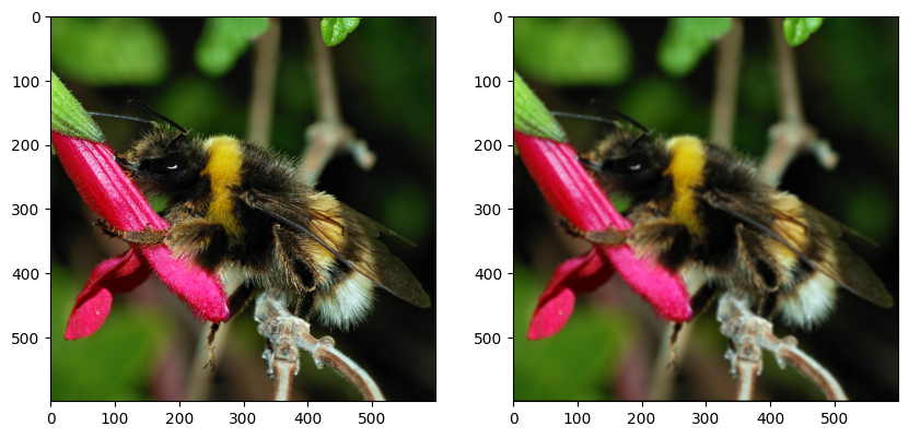
- Define una capa Conv2D con 3 filtros (5x5) que calculen la función identidad (preserven la imagen de entrada sin mezclar los colores).
- Cambia el stride a 2. ¿Cuál es el tamaño de la imagen de salida?
- Cambia el padding a VALID. ¿Qué se observa?
def my_init(shape=(5, 5, 3, 3), dtype=None):
array = np.zeros(shape=shape, dtype="float32")
array[2, 2] = np.eye(3)
return array
conv_strides_same = Conv2D(filters=3, kernel_size=5, strides=2,
padding="same", kernel_initializer=my_init,
input_shape=(None, None, 3))
conv_strides_valid = Conv2D(filters=3, kernel_size=5, strides=2,
padding="valid",
kernel_initializer=my_init)
img_in = np.expand_dims(sample_image, 0)
img_out_same = conv_strides_same(img_in)[0].numpy()
img_out_valid = conv_strides_valid(img_in)[0].numpy()
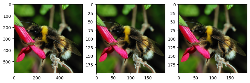
print("Shape of original image:", sample_image.shape)
print("Shape of result with SAME padding:", img_out_same.shape)
print("Shape of result with VALID padding:", img_out_valid.shape)
fig, (ax0, ax1, ax2) = plt.subplots(ncols=3, figsize=(12, 4))
ax0.imshow(img_in[0].astype(np.uint8))
ax1.imshow(img_out_same.astype(np.uint8))
ax2.imshow(img_out_valid.astype(np.uint8));/Users/aveloz/miniconda3/lib/python3.9/site-packages/keras/src/layers/convolutional/base_conv.py:107: UserWarning: Do not pass an `input_shape`/`input_dim` argument to a layer. When using Sequential models, prefer using an `Input(shape)` object as the first layer in the model instead.
super().__init__(activity_regularizer=activity_regularizer, **kwargs)Shape of original image: (600, 600, 3)
Shape of result with SAME padding: (300, 300, 3)
Shape of result with VALID padding: (298, 298, 3)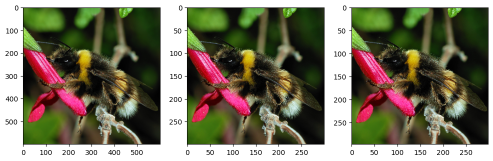
El stride de 2 divide el tamaño de la imagen a la mitad. En el caso de padding ‘VALID’, no agrega padding, por lo tanto el tamaño de la imagen de salida es el mismo que el tamaño original menos 2 debido al tamaño del kernel.
Detección de bordes en imágenes en escala de grises
# convert image to greyscale
grey_sample_image = sample_image.mean(axis=2)

# add the channel dimension even if it's only one channel so
# as to be consistent with Keras expectations.
grey_sample_image = grey_sample_image[:, :, np.newaxis]


# matplotlib does not like the extra dim for the color channel
# when plotting gray-level images. Let's use squeeze:
plt.imshow(np.squeeze(grey_sample_image.astype(np.uint8)),
           cmap=plt.cm.gray);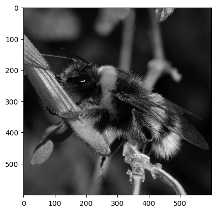
def my_init(shape, dtype=None):
    array = np.array([
        [0.0,  0.2, 0.0],
        [0.0, -0.2, 0.0],
        [0.0,  0.0, 0.0],
    ], dtype="float32")
    # adds two axis to match the required shape (3,3,1,1)
    return np.expand_dims(np.expand_dims(array,-1),-1)


conv_edge = Conv2D(kernel_size=(3,3), filters=1,
           padding="same", kernel_initializer=my_init,
           input_shape=(None, None, 1))

img_in = np.expand_dims(grey_sample_image, 0)
img_out = conv_edge(img_in).numpy()

fig, (ax0, ax1) = plt.subplots(ncols=2, figsize=(10, 5))
ax0.imshow(np.squeeze(img_in[0]).astype(np.uint8),
           cmap=plt.cm.gray);
ax1.imshow(np.squeeze(img_out[0]).astype(np.uint8),
           cmap=plt.cm.gray);

# vertical edge detection.
# Many other kernels work, for example differences
# of centered gaussians
#
# You may try with this filter as well
# np.array([
#         [ 0.1,  0.2,  0.1],
#         [ 0.0,  0.0,  0.0],
#         [-0.1, -0.2, -0.1],
#     ], dtype="float32")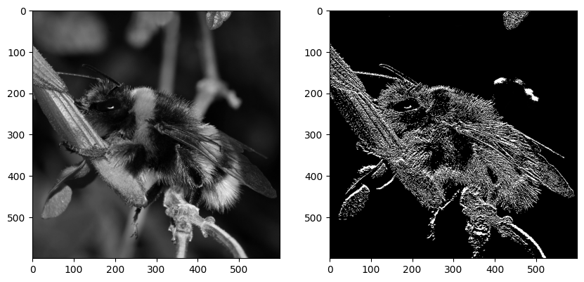
Pooling y strides con convoluciones
- Usa
MaxPool2Dpara aplicar un max pooling de 2x2 con strides de 2 a la imagen. ¿Cuál es el impacto en el tamaño de la imagen?
- Usa
AvgPool2Dpara aplicar un average pooling. - ¿Es posible calcular un max pooling y un average pooling con kernels elegidos a mano?
- Implementa un average pooling de 3x3 con una convolución regular
Conv2D, con strides, kernel y padding bien elegidos.
from tensorflow.keras.layers import MaxPool2D, AvgPool2Dmax_pool = MaxPool2D(2, strides=2)
img_in = np.expand_dims(sample_image, 0)
img_out = max_pool(img_in).numpy()
print("input shape:", img_in.shape)
print("output shape:", img_out.shape)
fig, (ax0, ax1) = plt.subplots(ncols=2, figsize=(10, 5))
ax0.imshow(img_in[0].astype('uint8'))
ax1.imshow(img_out[0].astype('uint8'));
# no es posible hacer un max pooling con kernels. Sí es posible hacer un average pooling.input shape: (1, 600, 600, 3)
output shape: (1, 300, 300, 3)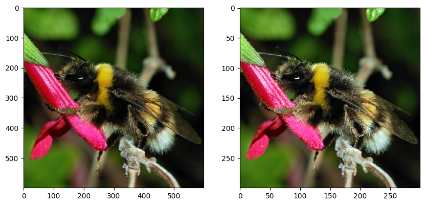
avg_pool = AvgPool2D(3, strides=3, input_shape=(None, None, 3))

img_in = np.expand_dims(sample_image, 0)
img_out_avg_pool = avg_pool(img_in).numpy()

def my_init(shape=(3, 3, 3, 3), dtype=None):
    array = np.zeros(shape=shape, dtype="float32")
    array[:, :, 0, 0] = 1 / 9.
    array[:, :, 1, 1] = 1 / 9.
    array[:, :, 2, 2] = 1 / 9.
    return array

conv_avg = Conv2D(kernel_size=3, filters=3, strides=3,
           padding="valid",
           kernel_initializer=my_init,
           input_shape=(None, None, 3))

img_out_conv = conv_avg(np.expand_dims(sample_image, 0)).numpy()

print("input shape:", img_in.shape)
print("output avg pool shape:", img_out_avg_pool.shape)
print("output conv shape:", img_out_conv.shape)

fig, (ax0, ax1, ax2) = plt.subplots(ncols=3, figsize=(10, 5))
ax0.imshow(img_in[0].astype('uint8'))
ax1.imshow(img_out_avg_pool[0].astype('uint8'))
ax2.imshow(img_out_conv[0].astype('uint8'));

print("Avg pool is similar to Conv ? -", np.allclose(img_out_avg_pool, img_out_conv))
input shape: (1, 600, 600, 3)
output avg pool shape: (1, 200, 200, 3)
output conv shape: (1, 200, 200, 3)
Avg pool is similar to Conv ? - True/Users/aveloz/miniconda3/lib/python3.9/site-packages/keras/src/layers/pooling/base_pooling.py:23: UserWarning: Do not pass an `input_shape`/`input_dim` argument to a layer. When using Sequential models, prefer using an `Input(shape)` object as the first layer in the model instead.
super().__init__(name=name, **kwargs)