Sistemas de Recomendación Neuronales con Retroalimentación Explícita

Objetivos:

• Comprender los sistemas de recomendación
  
• Construir diferentes arquitecturas de modelos utilizando Keras
  
• Recuperar y visualizar embeddings
  
• Incorporar información de metadatos como entrada del modelo

%matplotlib inline
import matplotlib.pyplot as plt
import numpy as np
import os

from zipfile import ZipFile
from urllib.request import urlretrieve

ML_100K_URL = "http://files.grouplens.org/datasets/movielens/ml-100k.zip"
ML_100K_FILENAME = ML_100K_URL.rsplit('/', 1)[1]
ML_100K_FOLDER = 'ml-100k'

if not os.path.exists(ML_100K_FILENAME):
    print('Downloading %s to %s...' % (ML_100K_URL, ML_100K_FILENAME))
    urlretrieve(ML_100K_URL, ML_100K_FILENAME)

if not os.path.exists(ML_100K_FOLDER):
    print('Extracting %s to %s...' % (ML_100K_FILENAME, ML_100K_FOLDER))
    ZipFile(ML_100K_FILENAME).extractall('.')

Archivo de Calificaciones

Cada línea contiene una película calificada:

• un usuario
  
• un ítem
  
• una calificación de 1 a 5 estrellas

import pandas as pd

raw_ratings = pd.read_csv(os.path.join(ML_100K_FOLDER, 'u.data'), sep='\t',
                      names=["user_id", "item_id", "rating", "timestamp"])
raw_ratings.head()

	user_id	item_id	rating	timestamp
0	196	242	3	881250949
1	186	302	3	891717742
2	22	377	1	878887116
3	244	51	2	880606923
4	166	346	1	886397596

# how many movies each user saw
user_movie_counts = raw_ratings.groupby('user_id')['item_id'].nunique()

plt.figure(figsize=(8, 5))
plt.hist(user_movie_counts, bins=30, edgecolor='black')
plt.xlabel('Movies seen per user')
plt.ylabel('Number of users');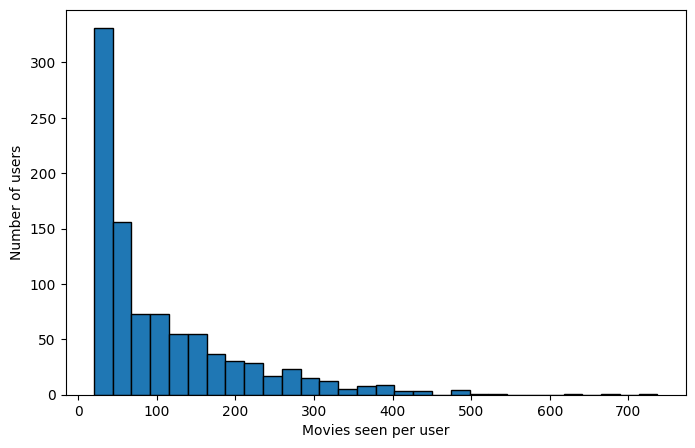

Archivo de Metadatos

El archivo de metadatos contiene información como el nombre de la película o la fecha en que fue estrenada. El archivo de películas incluye columnas que indican los géneros de cada película. Carguemos solo las primeras cinco columnas del archivo usando usecols.

m_cols = ['item_id', 'title', 'release_date', 'video_release_date', 'imdb_url']
items = pd.read_csv(os.path.join(ML_100K_FOLDER, 'u.item'), sep='|',
                    names=m_cols, usecols=range(5), encoding='latin-1')
items.head()

	item_id	title	release_date	video_release_date	imdb_url
0	1	Toy Story (1995)	01-Jan-1995	NaN	http://us.imdb.com/M/title-exact?Toy%20Story%2...
1	2	GoldenEye (1995)	01-Jan-1995	NaN	http://us.imdb.com/M/title-exact?GoldenEye%20(...
2	3	Four Rooms (1995)	01-Jan-1995	NaN	http://us.imdb.com/M/title-exact?Four%20Rooms%...
3	4	Get Shorty (1995)	01-Jan-1995	NaN	http://us.imdb.com/M/title-exact?Get%20Shorty%...
4	5	Copycat (1995)	01-Jan-1995	NaN	http://us.imdb.com/M/title-exact?Copycat%20(1995)

# Extract the release year as an integer value:

def extract_year(release_date):
    if hasattr(release_date, 'split'):
        components = release_date.split('-')
        if len(components) == 3:
            return int(components[2])
    # Missing value marker
    return 1920


items['release_year'] = items['release_date'].map(extract_year)
items.hist('release_year', bins=50)

array([[<Axes: title={'center': 'release_year'}>]], dtype=object)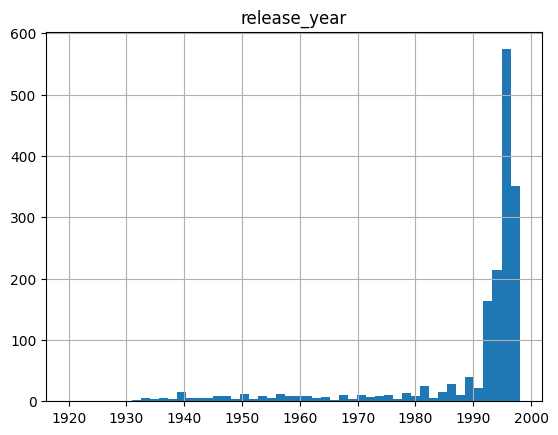

Complemento de los datos originales con los metadatos

all_ratings = pd.merge(items, raw_ratings)
all_ratings.head()

	item_id	title	release_date	video_release_date	imdb_url	release_year	user_id	rating	timestamp
0	1	Toy Story (1995)	01-Jan-1995	NaN	http://us.imdb.com/M/title-exact?Toy%20Story%2...	1995	308	4	887736532
1	1	Toy Story (1995)	01-Jan-1995	NaN	http://us.imdb.com/M/title-exact?Toy%20Story%2...	1995	287	5	875334088
2	1	Toy Story (1995)	01-Jan-1995	NaN	http://us.imdb.com/M/title-exact?Toy%20Story%2...	1995	148	4	877019411
3	1	Toy Story (1995)	01-Jan-1995	NaN	http://us.imdb.com/M/title-exact?Toy%20Story%2...	1995	280	4	891700426
4	1	Toy Story (1995)	01-Jan-1995	NaN	http://us.imdb.com/M/title-exact?Toy%20Story%2...	1995	66	3	883601324

• el número de usuarios
  
• el número de ítems
  
• la distribución de calificaciones
  
• la popularidad de cada película

min_user_id = all_ratings['user_id'].min()
max_user_id = all_ratings['user_id'].max()
print(min_user_id, max_user_id, all_ratings.shape)

1 943 (100000, 9)

min_item_id = all_ratings['item_id'].min()
max_item_id = all_ratings['item_id'].max()
print(min_item_id, max_item_id)

1 1682

all_ratings['rating'].describe()

count    100000.000000
mean          3.529860
std           1.125674
min           1.000000
25%           3.000000
50%           4.000000
75%           4.000000
max           5.000000
Name: rating, dtype: float64

Popularidad = n° de ratings que recibe una película

popularity = all_ratings.groupby('item_id').size().reset_index(name='popularity')
items = pd.merge(popularity, items)
items.nlargest(10, 'popularity')

	item_id	popularity	title	release_date	video_release_date	imdb_url	release_year
49	50	583	Star Wars (1977)	01-Jan-1977	NaN	http://us.imdb.com/M/title-exact?Star%20Wars%2...	1977
257	258	509	Contact (1997)	11-Jul-1997	NaN	http://us.imdb.com/Title?Contact+(1997/I)	1997
99	100	508	Fargo (1996)	14-Feb-1997	NaN	http://us.imdb.com/M/title-exact?Fargo%20(1996)	1997
180	181	507	Return of the Jedi (1983)	14-Mar-1997	NaN	http://us.imdb.com/M/title-exact?Return%20of%2...	1997
293	294	485	Liar Liar (1997)	21-Mar-1997	NaN	http://us.imdb.com/Title?Liar+Liar+(1997)	1997
285	286	481	English Patient, The (1996)	15-Nov-1996	NaN	http://us.imdb.com/M/title-exact?English%20Pat...	1996
287	288	478	Scream (1996)	20-Dec-1996	NaN	http://us.imdb.com/M/title-exact?Scream%20(1996)	1996
0	1	452	Toy Story (1995)	01-Jan-1995	NaN	http://us.imdb.com/M/title-exact?Toy%20Story%2...	1995
299	300	431	Air Force One (1997)	01-Jan-1997	NaN	http://us.imdb.com/M/title-exact?Air+Force+One...	1997
120	121	429	Independence Day (ID4) (1996)	03-Jul-1996	NaN	http://us.imdb.com/M/title-exact?Independence%...	1996

items["title"][49]

'Star Wars (1977)'

indexed_items = items.set_index('item_id')
indexed_items["title"][50]

'Star Wars (1977)'

all_ratings = pd.merge(popularity, all_ratings)
all_ratings.describe()

	item_id	popularity	video_release_date	release_year	user_id	rating	timestamp
count	100000.000000	100000.000000	0.0	100000.000000	100000.00000	100000.000000	1.000000e+05
mean	425.530130	168.071900	NaN	1987.950100	462.48475	3.529860	8.835289e+08
std	330.798356	121.784558	NaN	14.169558	266.61442	1.125674	5.343856e+06
min	1.000000	1.000000	NaN	1920.000000	1.00000	1.000000	8.747247e+08
25%	175.000000	71.000000	NaN	1986.000000	254.00000	3.000000	8.794487e+08
50%	322.000000	145.000000	NaN	1994.000000	447.00000	4.000000	8.828269e+08
75%	631.000000	239.000000	NaN	1996.000000	682.00000	4.000000	8.882600e+08
max	1682.000000	583.000000	NaN	1998.000000	943.00000	5.000000	8.932866e+08

all_ratings.head()

	item_id	popularity	title	release_date	video_release_date	imdb_url	release_year	user_id	rating	timestamp
0	1	452	Toy Story (1995)	01-Jan-1995	NaN	http://us.imdb.com/M/title-exact?Toy%20Story%2...	1995	308	4	887736532
1	1	452	Toy Story (1995)	01-Jan-1995	NaN	http://us.imdb.com/M/title-exact?Toy%20Story%2...	1995	287	5	875334088
2	1	452	Toy Story (1995)	01-Jan-1995	NaN	http://us.imdb.com/M/title-exact?Toy%20Story%2...	1995	148	4	877019411
3	1	452	Toy Story (1995)	01-Jan-1995	NaN	http://us.imdb.com/M/title-exact?Toy%20Story%2...	1995	280	4	891700426
4	1	452	Toy Story (1995)	01-Jan-1995	NaN	http://us.imdb.com/M/title-exact?Toy%20Story%2...	1995	66	3	883601324

train / test split

from sklearn.model_selection import train_test_split

ratings_train, ratings_test = train_test_split(
    all_ratings, test_size=0.2, random_state=0)

user_id_train = np.array(ratings_train['user_id'])
item_id_train = np.array(ratings_train['item_id'])
rating_train = np.array(ratings_train['rating'])

user_id_test = np.array(ratings_test['user_id'])
item_id_test = np.array(ratings_test['item_id'])
rating_test = np.array(ratings_test['rating'])

len(np.unique(user_id_test))

943

Retroalimentación explícita: predicción de calificaciones supervisada

Para cada par de (usuario, ítem) se intenta predecir la calificación que el usuario daría al ítem.

Este es el esquema clásico para construir sistemas de recomendación a partir de datos offline utilizando una señal de supervisión explícita.

Predicción de calificaciones como un problema de regresión

El siguiente código implementa la siguiente arquitectura:

from tensorflow.keras.layers import Embedding, Flatten, Dense, Dropout
from tensorflow.keras.layers import Dot
from tensorflow.keras.models import Model

# For each sample we input the integer identifiers
# of a single user and a single item
class RegressionModel(Model):
    def __init__(self, embedding_size, max_user_id, max_item_id):
        super().__init__()
        
        self.user_embedding = Embedding(output_dim=embedding_size,
                                        input_dim=max_user_id + 1,
                                        name='user_embedding')
        self.item_embedding = Embedding(output_dim=embedding_size,
                                        input_dim=max_item_id + 1,
                                        name='item_embedding')
        
        # The following two layers don't have parameters.
        self.flatten = Flatten()
        self.dot = Dot(axes=1)
        
    def call(self, inputs):
        user_inputs = inputs[0]
        item_inputs = inputs[1]
        
        user_vecs = self.flatten(self.user_embedding(user_inputs))
        item_vecs = self.flatten(self.item_embedding(item_inputs))
        
        y = self.dot([user_vecs, item_vecs])
        return y


model = RegressionModel(64, max_user_id, max_item_id)
model.compile(optimizer="adam", loss='mae')

# Useful for debugging the output shape of model
initial_train_preds = model.predict([user_id_train, item_id_train])
initial_train_preds.shape

2500/2500 ━━━━━━━━━━━━━━━━━━━━ 1s 399us/step

(80000, 1)

Error del modelo

Usando initial_train_preds, calcula los errores del modelo: - el error absoluto medio - el error cuadrático medio

La conversión de una serie de pandas a un arreglo numpy suele ser implícita, pero puedes usar rating_train.values para hacerlo explícitamente. Asegúrese de monitorear las dimensiones de cada objeto mediante object.shape.

squared_differences = np.square(initial_train_preds[:,0] - rating_train)
absolute_differences = np.abs(initial_train_preds[:,0] - rating_train)

print("Random init MSE: %0.3f" % np.mean(squared_differences))
print("Random init MAE: %0.3f" % np.mean(absolute_differences))

# You may also use sklearn metrics to do so using scikit-learn:

from sklearn.metrics import mean_absolute_error, mean_squared_error

print("Random init MSE: %0.3f" % mean_squared_error(initial_train_preds, rating_train))
print("Random init MAE: %0.3f" % mean_absolute_error(initial_train_preds, rating_train))

Random init MSE: 13.719
Random init MAE: 3.529
Random init MSE: 13.719
Random init MAE: 3.529

Monitoreo de ejecución

Keras permite monitorear varias variables durante el entrenamiento.

El objeto history.history devuelto por la función model.fit es un diccionario que contiene la pérdida de entrenamiento ('loss') y la pérdida de validación 'val_loss' después de cada época.

%%time

# Training the model
history = model.fit([user_id_train, item_id_train], rating_train,
                    batch_size=64, epochs=10, validation_split=0.1,
                    shuffle=True)

Epoch 1/10

1125/1125 ━━━━━━━━━━━━━━━━━━━━ 2s 1ms/step - loss: 3.3031 - val_loss: 1.0389

Epoch 2/10

1125/1125 ━━━━━━━━━━━━━━━━━━━━ 1s 1ms/step - loss: 0.9024 - val_loss: 0.7944

Epoch 3/10

1125/1125 ━━━━━━━━━━━━━━━━━━━━ 1s 998us/step - loss: 0.7565 - val_loss: 0.7696

Epoch 4/10

1125/1125 ━━━━━━━━━━━━━━━━━━━━ 1s 1ms/step - loss: 0.7285 - val_loss: 0.7613

Epoch 5/10

1125/1125 ━━━━━━━━━━━━━━━━━━━━ 1s 1ms/step - loss: 0.7040 - val_loss: 0.7487

Epoch 6/10

1125/1125 ━━━━━━━━━━━━━━━━━━━━ 2s 1ms/step - loss: 0.6831 - val_loss: 0.7406

Epoch 7/10

1125/1125 ━━━━━━━━━━━━━━━━━━━━ 1s 1ms/step - loss: 0.6585 - val_loss: 0.7450

Epoch 8/10

1125/1125 ━━━━━━━━━━━━━━━━━━━━ 1s 1ms/step - loss: 0.6401 - val_loss: 0.7425

Epoch 9/10

1125/1125 ━━━━━━━━━━━━━━━━━━━━ 1s 963us/step - loss: 0.6216 - val_loss: 0.7358

Epoch 10/10

1125/1125 ━━━━━━━━━━━━━━━━━━━━ 1s 920us/step - loss: 0.5941 - val_loss: 0.7403

CPU times: user 14.6 s, sys: 4.05 s, total: 18.6 s

Wall time: 12.9 s

plt.plot(history.history['loss'], label='train')
plt.plot(history.history['val_loss'], label='validation')
plt.ylim(0, 2)
plt.legend(loc='best')
plt.title('Loss');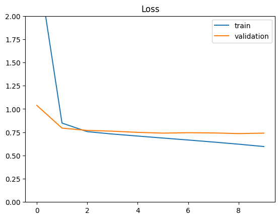

Ahora el modelo está entrenado. El MSE y el MAE es:

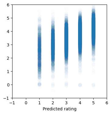
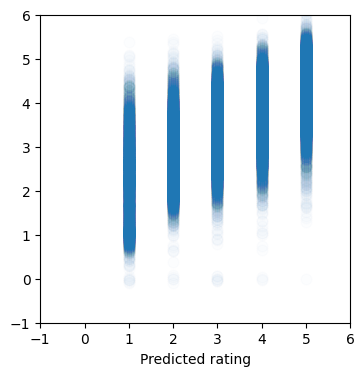
def plot_predictions(y_true, y_pred):
    plt.figure(figsize=(4, 4))
    plt.xlim(-1, 6)
    plt.xlabel("True rating")
    plt.ylim(-1, 6)
    plt.xlabel("Predicted rating")
    plt.scatter(y_true, y_pred, s=60, alpha=0.01)

from sklearn.metrics import mean_squared_error
from sklearn.metrics import mean_absolute_error

test_preds = model.predict([user_id_test, item_id_test])
print("Final test MSE: %0.3f" % mean_squared_error(test_preds, rating_test))
print("Final test MAE: %0.3f" % mean_absolute_error(test_preds, rating_test))
plot_predictions(rating_test, test_preds)

625/625 ━━━━━━━━━━━━━━━━━━━━ 0s 420us/step

Final test MSE: 0.903

Final test MAE: 0.735

train_preds = model.predict([user_id_train, item_id_train])
print("Final train MSE: %0.3f" % mean_squared_error(train_preds, rating_train))
print("Final train MAE: %0.3f" % mean_absolute_error(train_preds, rating_train))
plot_predictions(rating_train, train_preds)

2500/2500 ━━━━━━━━━━━━━━━━━━━━ 1s 324us/step

Final train MSE: 0.622

Final train MAE: 0.576

Embeddings

• Es posible obtener los embeddings simplemente utilizando la función de Keras model.get_weights, la cual retorna todos los parámetros entrenables del modelo.
• Los pesos se devuelven en el mismo orden en que fueron construidos en el modelo.
• ¿Cuál es el número total de parámetros?

# weights and shape
weights = model.get_weights()
[w.shape for w in weights]

[(944, 64), (1683, 64)]

model.summary()

Model: "regression_model"

┏━━━━━━━━━━━━━━━━━━━━━━━━━━━━━━━━━┳━━━━━━━━━━━━━━━━━━━━━━━━┳━━━━━━━━━━━━━━━┓
┃ Layer (type)                    ┃ Output Shape           ┃       Param # ┃
┡━━━━━━━━━━━━━━━━━━━━━━━━━━━━━━━━━╇━━━━━━━━━━━━━━━━━━━━━━━━╇━━━━━━━━━━━━━━━┩
│ user_embedding (Embedding)      │ (32, 64)               │        60,416 │
├─────────────────────────────────┼────────────────────────┼───────────────┤
│ item_embedding (Embedding)      │ (32, 64)               │       107,712 │
├─────────────────────────────────┼────────────────────────┼───────────────┤
│ flatten (Flatten)               │ (32, 64)               │             0 │
├─────────────────────────────────┼────────────────────────┼───────────────┤
│ dot (Dot)                       │ (32, 1)                │             0 │
└─────────────────────────────────┴────────────────────────┴───────────────┘

 Total params: 504,386 (1.92 MB)

 Trainable params: 168,128 (656.75 KB)

 Non-trainable params: 0 (0.00 B)

 Optimizer params: 336,258 (1.28 MB)

user_embeddings = weights[0]
item_embeddings = weights[1]

item_id = 181
print(f"Title for item_id={item_id}: {indexed_items['title'][item_id]}")

Title for item_id=181: Return of the Jedi (1983)

print(f"Embedding vector for item_id={item_id}")
print(item_embeddings[item_id])
print("shape:", item_embeddings[item_id].shape)

Embedding vector for item_id=181
[-0.13881622 -0.39279363 -0.4542818  -0.15036431 -0.07021406 -0.25858968
  0.3607689   0.35744905  0.40252867 -0.208011    0.08645177 -0.39484358
  0.40317655 -0.46558443 -0.39921615 -0.1384621  -0.4389023  -0.2775312
  0.02858883 -0.31169248 -0.12770256 -0.4184476   0.01467377 -0.1406344
 -0.530684   -0.14433524  0.20867957 -0.09543318  0.07717139  0.22346267
  0.48144048 -0.18085825 -0.3629786   0.13675222  0.3730956   0.38976803
  0.23840211 -0.21369277  0.23929588 -0.40205938  0.20967337  0.19232649
 -0.36350164 -0.0006811  -0.31449977  0.42901668  0.04440717 -0.04404833
 -0.25014856  0.30311036 -0.32103804 -0.36157265 -0.17517619  0.48115864
  0.27598906 -0.41375706  0.56592494  0.18957186 -0.02910222  0.52749366
  0.5087423   0.01733684 -0.37870777 -0.39084676]
shape: (64,)

Encontrar ítems similares

Buscar los k ítems más similares a un punto en el espacio de embeddings.

• Escribiremos una función para calcular la similitud del coseno entre dos puntos en el espacio de embeddings.
• Verificaremos las similitudes entre películas populares.

Notas: - Usar np.linalg.norm para calcular la norma de un vector. - La función de numpy np.argsort(...) permite obtener los índices ordenados de un vector. - items["name"][idxs] retorna los nombres de los ítems indexados por el arreglo idxs.

EPSILON = 1e-07 # to avoid division by 0.

def cosine(x, y):
    dot_products = np.dot(x, y.T)
    norm_products = np.linalg.norm(x) * np.linalg.norm(y)
    return dot_products / (norm_products + EPSILON)

def print_similarity(item_a, item_b, item_embeddings, titles):
    print(titles[item_a])
    print(titles[item_b])
    similarity = cosine(item_embeddings[item_a],
                        item_embeddings[item_b])
    print(f"Cosine similarity: {similarity:.3}")
    
print_similarity(50, 181, item_embeddings, indexed_items["title"])

Star Wars (1977)
Return of the Jedi (1983)
Cosine similarity: 0.915

print_similarity(181, 288, item_embeddings, indexed_items["title"])

Return of the Jedi (1983)
Scream (1996)
Cosine similarity: 0.814

print_similarity(181, 1, item_embeddings, indexed_items["title"])

Return of the Jedi (1983)
Toy Story (1995)
Cosine similarity: 0.832

print_similarity(181, 181, item_embeddings, indexed_items["title"])

Return of the Jedi (1983)
Return of the Jedi (1983)
Cosine similarity: 1.0

def cosine_similarities(item_id, item_embeddings):
    """Compute similarities between item_id and all items embeddings"""
    query_vector = item_embeddings[item_id]
    dot_products = item_embeddings @ query_vector

    query_vector_norm = np.linalg.norm(query_vector)
    all_item_norms = np.linalg.norm(item_embeddings, axis=1)
    norm_products = query_vector_norm * all_item_norms
    return dot_products / (norm_products + EPSILON)


similarities = cosine_similarities(181, item_embeddings)
similarities

array([0.0499818 , 0.8316962 , 0.7319682 , ..., 0.7540205 , 0.84227914,
       0.6886554 ], dtype=float32)

plt.hist(similarities, bins=30);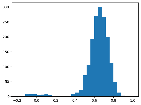

def most_similar(item_id, item_embeddings, titles, top_n=30):
    sims = cosine_similarities(item_id, item_embeddings)
    sorted_indexes = np.argsort(sims)[::-1]
    idxs = sorted_indexes[0:top_n]
    return list(zip(idxs, titles[idxs], sims[idxs]))

most_similar(50, item_embeddings, indexed_items["title"], top_n=10)

[(50, 'Star Wars (1977)', 0.99999994),
 (181, 'Return of the Jedi (1983)', 0.9154532),
 (172, 'Empire Strikes Back, The (1980)', 0.9115436),
 (1681, 'You So Crazy (1994)', 0.8846905),
 (12, 'Usual Suspects, The (1995)', 0.87451434),
 (1550, 'Destiny Turns on the Radio (1995)', 0.8683016),
 (127, 'Godfather, The (1972)', 0.86770046),
 (174, 'Raiders of the Lost Ark (1981)', 0.86769),
 (96, 'Terminator 2: Judgment Day (1991)', 0.8612536),
 (183, 'Alien (1979)', 0.8609332)]

items[items['title'].str.contains("Star Trek")]

	item_id	popularity	title	release_date	video_release_date	imdb_url	release_year
221	222	365	Star Trek: First Contact (1996)	22-Nov-1996	NaN	http://us.imdb.com/M/title-exact?Star%20Trek:%...	1996
226	227	161	Star Trek VI: The Undiscovered Country (1991)	01-Jan-1991	NaN	http://us.imdb.com/M/title-exact?Star%20Trek%2...	1991
227	228	244	Star Trek: The Wrath of Khan (1982)	01-Jan-1982	NaN	http://us.imdb.com/M/title-exact?Star%20Trek:%...	1982
228	229	171	Star Trek III: The Search for Spock (1984)	01-Jan-1984	NaN	http://us.imdb.com/M/title-exact?Star%20Trek%2...	1984
229	230	199	Star Trek IV: The Voyage Home (1986)	01-Jan-1986	NaN	http://us.imdb.com/M/title-exact?Star%20Trek%2...	1986
379	380	116	Star Trek: Generations (1994)	01-Jan-1994	NaN	http://us.imdb.com/M/title-exact?Star%20Trek:%...	1994
448	449	117	Star Trek: The Motion Picture (1979)	01-Jan-1979	NaN	http://us.imdb.com/M/title-exact?Star%20Trek:%...	1979
449	450	63	Star Trek V: The Final Frontier (1989)	01-Jan-1989	NaN	http://us.imdb.com/M/title-exact?Star%20Trek%2...	1989

most_similar(227, item_embeddings, indexed_items["title"], top_n=10)

[(227, 'Star Trek VI: The Undiscovered Country (1991)', 1.0000001),
 (228, 'Star Trek: The Wrath of Khan (1982)', 0.8696675),
 (1046, 'Malice (1993)', 0.8671569),
 (230, 'Star Trek IV: The Voyage Home (1986)', 0.8560517),
 (1483, 'Man in the Iron Mask, The (1998)', 0.8526243),
 (354, 'Wedding Singer, The (1998)', 0.8507102),
 (94, 'Home Alone (1990)', 0.8461486),
 (1431, 'Legal Deceit (1997)', 0.84468913),
 (257, 'Men in Black (1997)', 0.8440615),
 (1339, 'Stefano Quantestorie (1993)', 0.8437165)]

Las similitudes no siempre tienen sentido: el número de valoraciones es bajo y el embedding no captura automáticamente las relaciones semánticas en ese contexto. Se podrían obtener mejores representaciones con mayor cantidad de valoraciones, menos sobreajuste en los modelos o quizás con una función de pérdida más adecuada, como aquellas basadas en retroalimentación implícita.

Visualización de embeddings usando TSNE

from sklearn.manifold import TSNE

item_tsne = TSNE(perplexity=30).fit_transform(item_embeddings)

import matplotlib.pyplot as plt

plt.figure(figsize=(10, 10))
plt.scatter(item_tsne[:, 0], item_tsne[:, 1]);
plt.xticks(()); plt.yticks(());
plt.show()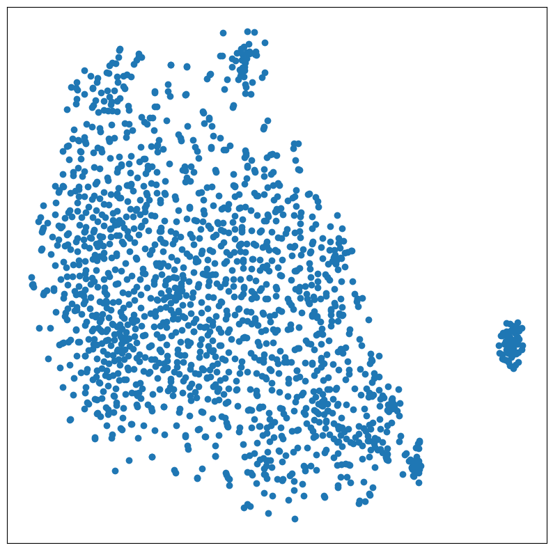

# %pip install -q plotly

import plotly.express as px

tsne_df = pd.DataFrame(item_tsne, columns=["tsne_1", "tsne_2"])
tsne_df["item_id"] = np.arange(item_tsne.shape[0])
tsne_df = tsne_df.merge(items.reset_index())

px.scatter(tsne_df, x="tsne_1", y="tsne_2",
           color="popularity",
           hover_data=["item_id", "title",
                       "release_year", "popularity"])

Unable to display output for mime type(s): application/vnd.plotly.v1+json

Alternativamente - UMAP Uniform Manifold Approximation and Projection:

# %pip install umap-learn

import umap

item_umap = umap.UMAP().fit_transform(item_embeddings)
plt.figure(figsize=(10, 10))
plt.scatter(item_umap[:, 0], item_umap[:, 1]);
plt.xticks(()); plt.yticks(());
plt.show()

Sistema de recomendación profundo

from tensorflow.keras.layers import Concatenate

# For each sample we input the integer identifiers
# of a single user and a single item
class DeepRegressionModel(Model):

    def __init__(self, embedding_size, max_user_id, max_item_id):
        super().__init__()

        self.user_embedding = Embedding(
            output_dim=embedding_size,
            input_dim=max_user_id + 1,
            name='user_embedding'
        )
        self.item_embedding = Embedding(
            output_dim=embedding_size,
            input_dim=max_item_id + 1,
            name='item_embedding'
        )

        # The following two layers don't have parameters.
        self.flatten = Flatten()
        self.concat = Concatenate()

        ## possible error: Dropout too high, preventing any training
        self.dropout = Dropout(0.5)
        self.dense1 = Dense(64, activation="relu")
        self.dense2 = Dense(1)

    def call(self, inputs, training=False):
        user_inputs = inputs[0]
        item_inputs = inputs[1]

        user_vecs = self.flatten(self.user_embedding(user_inputs))
        item_vecs = self.flatten(self.item_embedding(item_inputs))

        input_vecs = self.concat([user_vecs, item_vecs])

        y = self.dropout(input_vecs, training=training)
        y = self.dense1(y)
        y = self.dropout(y, training=training)
        y = self.dense2(y)

        return y

model = DeepRegressionModel(64, max_user_id, max_item_id)
model.compile(optimizer='adam', loss='mae')

initial_train_preds = model.predict([user_id_train, item_id_train])

2500/2500 ━━━━━━━━━━━━━━━━━━━━ 1s 360us/step

%%time
history = model.fit([user_id_train, item_id_train], rating_train,
                    batch_size=64, epochs=10, validation_split=0.1,
                    shuffle=True)

Epoch 1/10

1125/1125 ━━━━━━━━━━━━━━━━━━━━ 2s 1ms/step - loss: 1.5973 - val_loss: 0.7786

Epoch 2/10

1125/1125 ━━━━━━━━━━━━━━━━━━━━ 1s 1ms/step - loss: 0.8779 - val_loss: 0.7660

Epoch 3/10

1125/1125 ━━━━━━━━━━━━━━━━━━━━ 1s 1ms/step - loss: 0.8470 - val_loss: 0.7598

Epoch 4/10

1125/1125 ━━━━━━━━━━━━━━━━━━━━ 1s 1ms/step - loss: 0.8178 - val_loss: 0.7583

Epoch 5/10

1125/1125 ━━━━━━━━━━━━━━━━━━━━ 1s 1ms/step - loss: 0.7942 - val_loss: 0.7470

Epoch 6/10

1125/1125 ━━━━━━━━━━━━━━━━━━━━ 1s 1ms/step - loss: 0.7759 - val_loss: 0.7495

Epoch 7/10

1125/1125 ━━━━━━━━━━━━━━━━━━━━ 1s 1ms/step - loss: 0.7647 - val_loss: 0.7427

Epoch 8/10

1125/1125 ━━━━━━━━━━━━━━━━━━━━ 1s 1ms/step - loss: 0.7494 - val_loss: 0.7424

Epoch 9/10

1125/1125 ━━━━━━━━━━━━━━━━━━━━ 1s 1ms/step - loss: 0.7423 - val_loss: 0.7355

Epoch 10/10

1125/1125 ━━━━━━━━━━━━━━━━━━━━ 1s 1ms/step - loss: 0.7344 - val_loss: 0.7359

CPU times: user 15.5 s, sys: 3.9 s, total: 19.4 s

Wall time: 13.5 s

plt.plot(history.history['loss'], label='train')
plt.plot(history.history['val_loss'], label='validation')
plt.ylim(0.5, 0.8)
plt.legend(loc='best')
plt.title('Loss');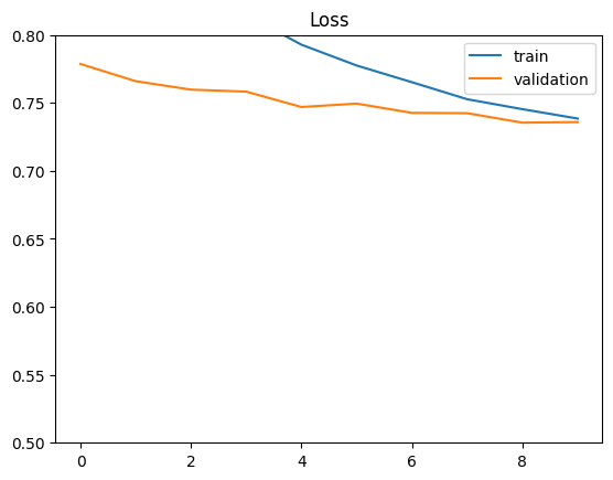

train_preds = model.predict([user_id_train, item_id_train])
print("Final train MSE: %0.3f" % mean_squared_error(train_preds, rating_train))
print("Final train MAE: %0.3f" % mean_absolute_error(train_preds, rating_train))

2500/2500 ━━━━━━━━━━━━━━━━━━━━ 1s 348us/step

Final train MSE: 0.835

Final train MAE: 0.706

test_preds = model.predict([user_id_test, item_id_test])
print("Final test MSE: %0.3f" % mean_squared_error(test_preds, rating_test))
print("Final test MAE: %0.3f" % mean_absolute_error(test_preds, rating_test))

625/625 ━━━━━━━━━━━━━━━━━━━━ 0s 359us/step

Final test MSE: 0.889

Final test MAE: 0.735

El desempeño de este modelo no es significativamente mejor que el modelo anterior, pero se puede notar que la diferencia entre el conjunto de entrenamiento y el de prueba es menor, probablemente gracias al uso de dropout, que ayuda a reducir el sobreajuste y mejora la generalización.

Además, este modelo es más flexible en el sentido de que se puede extender para incluir metadatos y construir sistemas de recomendación híbridos.